Femtolab Data Analysis

The Femtolab_Data_Analysis app is developed by Dr. Zhipeng Huang. It is a MATLAB based graphical user interface (GUI) for quickly analysing and visualizing the sum-frequency generation (SFG) spectroscopy and time-of-flight (TOF) mass spectroscopy data.

The application documentation for the main branch is automatically published on this project’s GitHub Page.

Set Up

Follow these steps to set up Femtolab_Data_Analysis:

1. Install MATLAB.

2. Clone or download the main branch to your local computer disk.

3. Add the Femtolab_Data_Analysis/ReadSFG folder and its subfolders to the MATLAB search path. Run MATLAB and type pathtool in the command window. There will be a window pop up for adding folders to the MATLAB search path.

Run the application

1. Type cmidaq_iteration in the MATLAB command window. The Femtolab_Data_Analysis app will be poped up.

2. Select the menu on the top left panel, click File -> Open mass spectrum data to choose the TOF mass spectroscopy data to be opened. It can open the .bin, .h5, .hdf5 file(s) collected by the LabView program for controlling the digitizer and digitial delay generator.

3. Select the File -> Open SFG data to choose the SFG data to be opened. It can open the .spe file(s) collected by the lightfield softeware for controlling the Princeton Instrument cameras and spectrographs. It can also open the .csv, .h5, .txt types of files.

4. When collecting the SFG spectrum, the background spectrum (collected by blocking the infrared beam path) can be either collected seperately or subtracted directly during the data collection. Therefore, there is a sub-window poping up to provide the option Would you like to substract the background and normalize the spectrum? after clicking the menu File -> Open SFG data. If the background spectrum is collected seperately, you can choose Subtract background only to subtract the background. If the background has been subtracted during the data collection, you then choose No.

5. The Subtract and normalize option is used for subtracting the background and normalize the spectrum with a referece sample specta (e.g. gold, quartz, etc.). The output result will be $I_{output}=\frac{I_{sam}-I_{sambkg}}{I_{ref}-I_{refbkg}}$ , where $I_{sam},I_{sambkg},I_{ref},I_{refbkg}$ are the sample SFG signal, sample SFG bakground signal, referece SFG signal, referece SFG background signal.

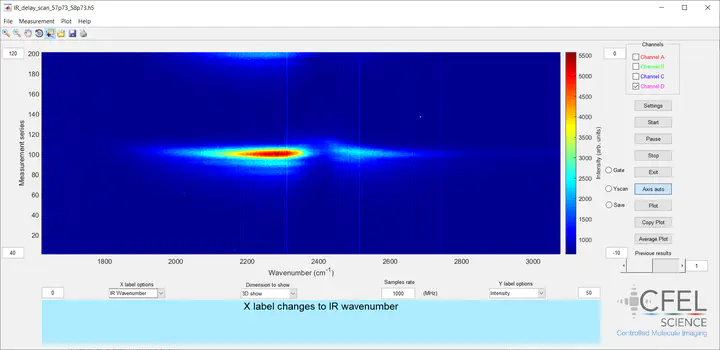
6. Once the spectrum is loaded, change the X label options located in the bottom left panel to SFG Wavelength. Click the Axis auto button located in the right middle panel to display the spectrum in the axis auto mode. It can be switched to the Maual axis mode by clicking the Axis auto button and type the axis range in the texbook neaby the two sides of the x and y axis.

7. The X label options provides several options to switch the x axis. The SFG Wavelength is to display the x axis in SFG wavelength mode. The SFG Photon Energy is to display the x axis in SFG Photon Energy mode. The IR Wavelength is to display the x axis in IR wavelength mode. The IR Wavenumber is to display the x axis in IR wavenumber mode. When swithing to the IR Wavelength or IR wavenumber mode, a subwindow will be poped up for typing the Enter up conversion center wavelength (nm). For our case we use the narrowband 800 nm as the up-conversion beam. The accurate value is measured by a spectrometer. The conversion between the different x axis mode is given by $X_{SFG Photon Energy} (eV)= \frac{1240}{X_{SFG Wavelength}(nm)}$ ; $X_{IR Wavelength} (nm)= \frac{1240}{\frac{1240}{X_{SFG Wavelength}(nm)}-\frac{1240}{X_{SFG Wavelength}(nm)}}$ ; $X_{IR Wavenumber} (cm^{-1}) = \frac{10^7}{X_{IR Wavelength} (nm)}$.

8. By clicking the Average Plot button, the displayed SFG specrtrum will be averaged if mutiple spectrum are opened.

9. By clicking the Copy Plot button, the displayed SFG specrtrum will be poped up and can be copied and saved to other format.

10. By sliding the Previous results button, it will display the SFG/TOF specrtrum of a certain indexed frame.

11. By clicking the Plot button, you will be reminded to select four data tips Click line to select four data tips: background is primary than gatedata, then press Return. The four data tips are used to selecte two data regions, one is for signal (peak) region, another one is for background region. Once the four data tips are selected, press return button in keyboard. It will then plot how the background subtracted signal region changes as a function of the measurment series. The proceed data will be saved in the MATLAB workspace.

12. Select the File -> Save rawdata workspace, the displayed the SFG spectrum is saved to the MATLAB workspace for further analysis.

13. Select the menu panel Plot -> Show all, the displayed panel will show all the loaded spectrum in our figure.

14. Select the menu panel Plot -> Filter outliers, it can remove the outliers of the spectrum shown in the display panel.

15. Select the menu panel Plot -> Undo Filtering, it will undo the outliers removal of the spectrum shown in the display panel.

16. Click the Help menu panel will display the email address where the questions can be sented for feedback.